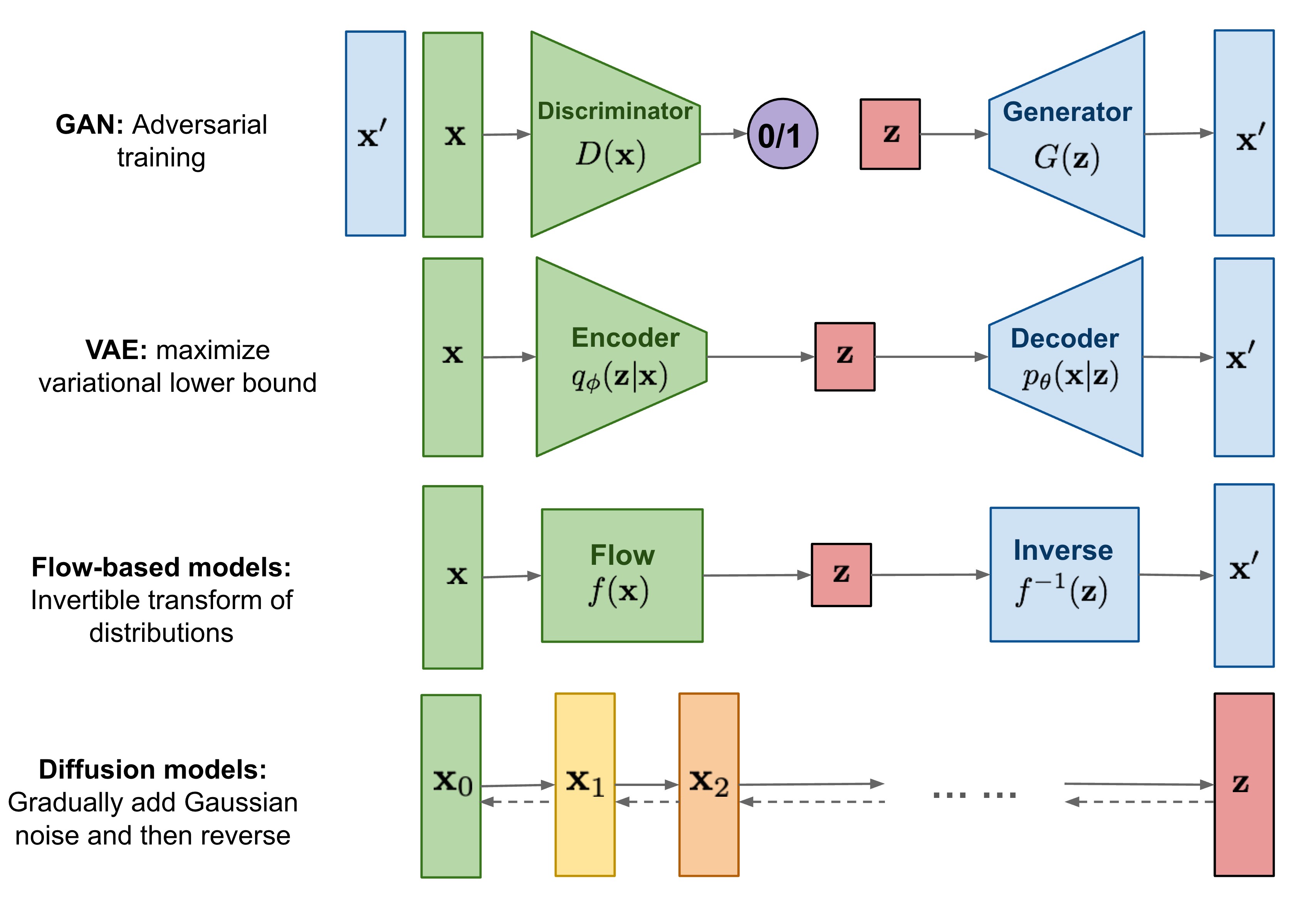
Generative Models
Generative modeling is a core building block across modern machine learning, from image synthesis to trajectory generation and world modeling.
This post reviews two dominant paradigms: generative adversarial networks (GANs) and diffusion models, and their variants.
1. What Is a Generative Model?
Given data \(x \sim p_\text{data}(x)\), a generative model learns an approximation \(p_\theta(x)\) such that:
- generates samples that resemble real data
- covers the full data distribution.
2. TODO: Variational Auto-Encoder (VAE)
3. Generative Adversarial Networks (GANs) [1]
3.1 Core Idea
GANs train two networks:
- A generator \(G\) generates synthetic samples (\(x = G(z)\)), given a noise variable input \(z\) who usually follows a standard normal distribution and introducespotential output diversity. It is trained to trick the discriminator to offer a high probability.
- Discriminator \(D\) outputs the probability of a given sample coming from the real dataset (\(D(x)\)). It is trained to distinguish the fake samples from the real ones.
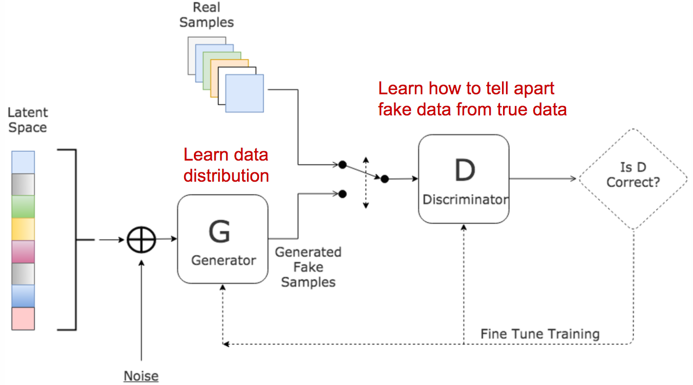
These two models compete against each other during the training process: the generator \(G\) is trying hard to trick the discriminator, while the critic model \(D\) is trying hard not to be cheated, which forms a zero-sum game.
Suppose \(p_r,p_g,p_z\) distributions over the real sample \(x\), generated sample \(x\) and random noise \(z\) (usually a standard normal distribution). The minimax objective is like:
\[\begin{aligned} \min_G \max_D L(G, D) = \mathbb{E}_{x \sim p_r}[\log D(x)] + \mathbb{E}_{z \sim p_z}[\log(1 - D(G(z)))] \\ = \mathbb{E}_{x \sim p_r}[\log D(x)] + \mathbb{E}_{x \sim p_g}[\log(1 - D(x)]. \end{aligned}\]3.2 What is the optimal value for \(D\)?
Examinte the best value for \(D\) by calulating the stationary point:
\[D^*(x) = \frac{p_r(x)}{p_r(x) + p_g(x)}.\]3.3 What does the loss function represent?
Given the optimal discriminator \(D^*\), find the relations between real and synthetic data distributions \(p_r\) and \(p_g\):
\[\begin{aligned} L(G, D^*) = \mathbb{E}_{x \sim p_r}[\log \frac{p_r(x)}{p_r(x)+p_g(x)}] + \mathbb{E}_{x \sim p_g}[\log \frac{p_g(x)}{p_r(x)+p_g(x)}] \\ = D_{KL}(p_r\|\frac{p_r+p_g}{2}) - \log2 + D_{KL}(p_g\|\frac{p_r+p_g}{2}) - \log2 \\ = 2D_{JS}(p_r \| p_g) - \log4. \end{aligned}\]3.4 TODO: Problems in GANs
- Hard to achieve Nash equilibrium
- Low dimensional supports
- Vanishing gradient
- Mode collapse
- Lack of a proper evaluation metric (unknown likelihood of \(p_g\))
3.5 Wasserstein GAN (WGAN) [2]
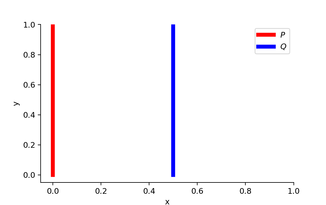
Wasserstein Distance is a measure of the distance between two probability distributions, which can be interpreted as the minimum energy cost of moving and transforming a pile of dirt in the shape of one probability distribution to the shape of the other distribution. When dealing with the continuous probability domain, the distance formula becomes:
\[W(p_r, p_g) = \inf_{\gamma \sim \Pi(p_r, p_g)} \mathbb{E}_{(x_1,x_2) \sim \gamma}[ \|x_1 - x_2\| ], \\\\\]where \(\tau(x_1,x_2)\) states the joint distribution that satisfies the boundary conditions of \(\int_{x_2} \gamma(x_1,x_2)dx_2 = p_r(x_1)\) and \(\int_{x_1} \gamma(x_1,x_2)dx_1 = p_g(x_2)\).
TODO: Why Wasserstein is better than JS or KL divergence?
Use Wasserstein distance as GAN loss function
It is intractable to exhaust all the possible joint distributions in \(\Pi(p_r, p_g)\) to compute \(\inf_{\gamma\sim \Pi(p_r, p_g)}\) . Thus the authors proposed a smart transformation of the formula based on the Kantorovich-Rubinstein duality to:
\[D_W(p_r, p_g) = \frac{1}{K} \sup_{\|f\| \le K} \mathbb{E}_{x\sim p_r}[f(x)] - \mathbb{E}_{x \sim p_g} [f(x)],\]where the real-valued function \(f: \mathbb{R} \to \mathbb{R}\) should be K-Lipschitz continuous. Read this blog for more about this duality transformation. In the modified Wasserstein GAN, the “discriminator” model is used to find a good function \(f_w\) parametrized by \(w \in W\) and the loss function is configured as measuring the Wasserstein distance between \(p_r\) and \(p_g\):
\[L(p_r,p_g) = D_W(p_r, p_g) = \max_{w \in W} \mathbb{E}_{x\sim p_r}[f_w(x)] - \mathbb{E}_{x \sim p_g} [f_w(x)].\]To maintain the K-Lipschitz continuity of function \(f_w\) during training, the paper presents a simple but very practical trick: After every gradient update, clamp the weights \(w\) to a small window, such as \([-0.01, 0.01]\).
3.6 Connections to Actor-Critic Methods [3]
The Mathematical Bridge: Bilevel Optimization
\[\begin{aligned} x^* = \arg \min_x F(x, y^*(x)) \quad\text{(Outer Opt.)} \\ y^*(x) = \arg \min_y f(x, y) \quad\text{(Inner Opt.)}. \end{aligned}\]| Component | GANs | Actor-Critic Methods |
|---|---|---|
| Outer Model (x) | Discriminator (\(D\)) | Critic (\(Q\)-function) |
| Outer Objective (F) | \(-L(G, D)\) | \(-\mathbb{E}_{s,a}[D_{KL}(\mathbb{E}_{r,s',a'}[r+\gamma Q(s', a')]|Q (s, a)]\) |
| Inner Model (y) | Generator (\(G\)) | Actor (Policy \(\pi\)) |
| Inner Objective (f) | \(-\mathbb{E}_{z\sim p_z}[\log D(G(z))]\) | \(-\mathbb{E}_{s \sim \mu,a\sim\pi}[Q(s, a)]\) |
GANs as a kind of Actor-Critic
For an RL environment with:
- State: stateless
- Action: generates an entire image
- Environment step: randomly decides to show either a real image of a generated image
- Reward: +1 if a real image is shown, 0 if the generated image is shown
reward/state does not depend on action.
4. Diffusion Models
Several diffusion-based generative models have been proposed with similar ideas underneath, including diffusion probabilistic models (DPM; Sohl-Dickstein et al., 2015), noise-conditioned score network (NCSN; Yang & Ermon, 2019), and denoising diffusion probabilistic models (DDPM; Ho et al. 2020).
4.1 Forward Diffusion Process: From Data to Noise
Given a data point sampled from a real data distribution \(x_0 \sim p_r(x)\), a forward diffusion process, we can gradually add small amount of Gaussian noise in \(T\) steps, producing a sequence os noisy samples \(x_1,\dots,x_T\). The step sizes are controlled by a variance schedule \({\beta_t \in (0,1)}_{t=1}^T\):
\[q(x_t|x_{t-1}) = \mathcal{N}(x_t;\sqrt{1-\beta_t}x_{t-1}, \beta_t\mathbf{I}), q(x_{0:T}|x_0) = \prod_{t=1}^T q(x_t|x_{t-1}).\]When \(T\to \infty\), \(x_T\) is equivalent to an isotropic Gaussian distribution.
Reparametrization tricks: from \(x_0\) to \(x_t\)
\[\begin{aligned} x_t = \sqrt{1-\beta_t}x_{t-1} + \sqrt{\beta_t} \epsilon_{t-1} \quad\text{;where $\epsilon_{t-1} \sim \mathcal{N}(\mathbf{0}, \mathbf{I})$} \\ = \sqrt{(1-\beta_t)(1-\beta_{t-1})}x_{t-2} + \sqrt{1-(1-\beta_t)(1-\beta_{t-1})} \bar{\epsilon}_{t-2} \quad\text{;where $\bar{\epsilon}_{t-2}$ merges two Gaussians} \\ = \dots \\ = \sqrt{\bar{\alpha}_t} x_0 + \sqrt{1-\bar{\alpha}_t} \epsilon \quad\text{;where $\epsilon \sim \mathcal{N}(\mathbf{0}, \mathbf{I})$}\\ q(x_t|x_0) = \mathcal{N}(x_t; \sqrt{\bar{\alpha}_t} x_0, (1-\bar{\alpha}_t)\mathbf{I}). \end{aligned}\]Connections with stochasitic gradient Langevin dynamics
Langevin dynamics is a concept from physics, developed for statistically modeling molecular systems. Combined with stochastic gradient descent, stochastic gradient Langevin dynamics (SGLD; Welling & Teh 2011) can produce samples from a probability density \(p(x)\) using only the gradients \(\nabla_x \log p(x)\) in a Markov chain of updates:
\[x_t = x_{t-1} + \Delta_t/2 \nabla_x \log p(x_{t-1}) + \sqrt{\Delta_t}\epsilon_t, \quad\text{where $\epsilon_{t} \sim \mathcal{N}(\mathbf{0}, \mathbf{I})$},\]where \(\Delta_t\) is the step size. When \(T \to \infty, \epsilon \to 0\), $x_T$ equals to the true probability \(p(x)\). The Gaussian noise avoids collapses into local minima.
4.2 Reverse Diffusion Process: From Noise to Data
If we can reverse the above process and sample from \(p_{\theta}(x_{t-1}\vert x_t)\), we will be able to recreate the true sample from a Gaussian noise input, \(x_T \sim \mathcal{N}(\mathbf{0}, \mathbf{I})\):
\[p_{\theta}(x_{t-1}|x_t) = \mathcal{N}(x_{t-1};\mu_{\theta}(x_t, t), \Sigma_\theta(x_t, t)), p_\theta(x_{0:T}) = p(x_T) \prod_{t=1}^T p_\theta(x_{t-1}|x_t).\]Distribution Representation 1: from \(x_t, x_0\) to \(x_{t-1}\)
It is noteworthy that the reverse conditional probability is tractable when conditioned on real sample \(x_0\) :
\[\begin{aligned} q(x_{t-1}|x_t, x_0) = \mathcal{N}(x_{t-1};\tilde{\mu}(x_t, x_0), \tilde{\beta}_t\mathbf{I}), \\ \tilde{\mu}(x_t, x_0) = \frac{\sqrt{1-\beta_t}( 1- \bar{\alpha}_{t-1})}{1-\bar{\alpha}_t} x_t + \frac{\sqrt{\bar{\alpha}_{t-1}}\beta_t}{1-\bar{\alpha}_t} x_0 \\ \tilde{\beta}_t = \frac{1-\bar{\alpha}_{t-1}}{1-\bar{\alpha}_t} \beta_t. \end{aligned}\]Distribution Representation 2: from \(x_t\) to \(x_{t-1}\)
From the reparametrization tricks above, we can replace \(x_0\) with \(x_t\):
\[\begin{aligned} \tilde{\mu}(x_t) = \frac{\sqrt{1-\beta_t}( 1- \bar{\alpha}_{t-1})}{1-\bar{\alpha}_t} x_t + \frac{\sqrt{\bar{\alpha}_{t-1}}\beta_t}{1-\bar{\alpha}_t}\frac{1}{\sqrt{\bar{\alpha}_t}} (x_t - \sqrt{1-\bar{\alpha}_t} \epsilon \\ = \frac{1}{\sqrt{1-\beta_t}} (x_t - \frac{\beta_t}{\sqrt{1-\bar{\alpha}_t}}\epsilon) \quad\text{;where $\bar{\alpha}_{t} = \bar{\alpha}_{t-1}(1-\beta_t)$} \end{aligned}\]The above derivations can be achieved by Bayesian rule, see this blog for details. We want to use a parametrized function \(\mu_{\theta}(x_t, t)\) to represent \(\tilde{\mu}(x_t)\). Since \(x_t\) is known during training, we only need to learn to predict noises \(\epsilon\) with \(\epsilon_\theta(x_t, t)\).
4.3 Training and Sampling Process
TODO: dervie VLB loss:
TODO: dervie NCSN loss:
TODO: dervie DDPM loss:
\[\begin{aligned} L_\text{DDPM} = \mathbb{E}_{x_0, t \sim [1, T], \epsilon}[\|\epsilon - \epsilon_\theta(x_t, t)\|^2 ] \\ = \mathbb{E}_{x_0, t \sim [1, T], \epsilon}[\|\epsilon - \epsilon_\theta(\sqrt{\bar{\alpha}_t}x_0 + \sqrt{1-\bar{\alpha}_t}\epsilon, t)\|^2 ] \\ \end{aligned}\]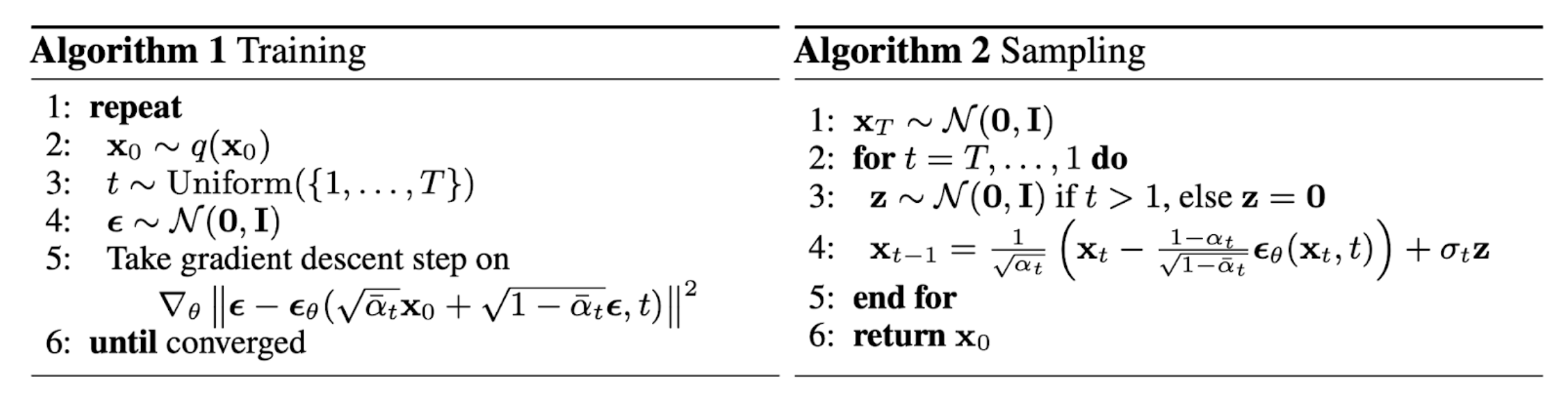
5. Flow-Matching Models
5.1 Mathematical Background
Forward Diffusion as Stochasitic Diffential Equation (SDE)
If we make the diffusion step \(\Delta t \to 0\) and the forward diffusion process becomes a stochastic differential equation (SDE):
\[dx = f(x,t)dt + g(t)dw\]where:
- \(w\) represents a Wiener process (i.e., Brownian random motion);
- \(f(\cdot, t)\) is called the drift;
- \(g(t)\) is called the diffusion term.
| Diffusion Methods | \(f(x, t)\) | \(g(t)\) |
|---|---|---|
| DDPM | \(-\frac{1}{2}\beta_tx\) | \(\sqrt{\beta_t}\) |
| NCSN | \(0\) | \(\sqrt{\frac{d\sigma_t^2}{dt}}\) |
By carefully designing noise scheduling \(\beta_t\) and \(\sigma_t\) , DDPM and NCSN can generate the same probability path \(\{p_t(x)\}\) and different SDEs are just different mathematical formulas to describe the same process,
Equivelance between SDE and Ordinary Differential Equation (ODE)
Song 2021 has proved that for any SDE, it has a corresponding ordinary differential equation (ODE) inducing the same \(p_t(x)\), which is called probability flow ODE with the following format: \(\frac{dx}{dt} = f(x,t) - \frac{1}{2}g(t)^2 \nabla_x \log p_t(x)\)
This connection transforms a random “walk” to a deterministic “flow” along the ODE trajectory, (1) easing the sampling process of the diffusion process (DDIM, Song 2021) and (2) inducing following simpler flow-matching methods.
5.2 Flow-Matching Methods
Probability flow ODE relies on a global score-based function \(\nabla_x \log p_t(x)\) to generate samples, which is difficult to learn. While flow-matching methods directly design a simple path from real data \(x_0\) to pure noise \(x_1\). The simplest path is a constant-speed motion \(x_t=(1-t)x_0 + tx_1\). We need to learn a parametrized function \(v_{\theta}(x_t, t)\) to match the real speed $x_1-x_0$.
5.3 Training and Sampling Process
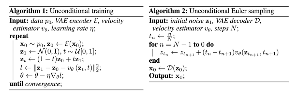
\(z\) and \(x\) can be the same space or \(z\) be the latent space and flow-matching happens on that space.
References
[1] Goodfellow, Ian, et al. “Generative Adversarial Nets.” Neurips, 2014.
[2] Martin Arjovsky, Soumith Chintala, and Léon Bottou. “Wasserstein GAN.” ICML, 2017.
[3] David Pfau, Oriol Vinyals. “Connecting Generative Adversarial Networks and Actor-Critic Methods.” arXiv, 2016.
[4] Calvin Luo. “Understanding Diffusion Models: A Unified Perspective.” arXiv, 2022.
TODO: unify references and hyperlinks in the blog.